Properties of drilling fluids

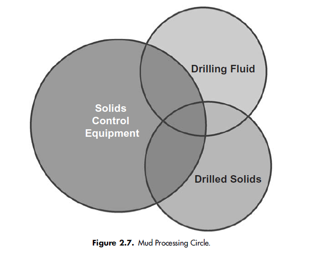
Just as the nature of drilling-fluid solids affects the efficiency of solids control equipment, the nature of the solids also plays an integral role in the properties of drilling fluids, which in turn affect the properties of the solids and the performance of the equipment. This intricate and very complex dynamic relationship among the solids, drilling fluid, and solids-control equipment is represented in Figure 2.7. Any change made to one of these affects the other two, and those in turn affect all three,and so on. To optimize a drilling operation, it is important to understand how the solids affect bulk mud properties, particularly rheology, hole cleaning, filtration, drilling rate (rate of penetration [ROP]), along with surface properties such as shale inhibition potential, lubricity, and wetting characteristics.

1.Rheology
Rheology is the study of the deformation and flow of matter. Viscosity is a measure of the resistance offered by that matter to a deforming force. Shear dominates most of the viscosity-related aspects of drilling operations. Because of that, shear viscosity (or simply, ‘‘viscosity’’) of drilling fluids is the property that is most commonly monitored and controlled. Retention of drilling fluid on cuttings is thought to be primarily a function of the viscosity of the mud and its wetting characteristics. Drilling fluids with elevated viscosity at high shear rates tend to exhibit greater retention of mud on cuttings and reduce the efficiency of high-shear devices like shale shakers [Lundie]. Conversely, elevated viscosity at low shear rates reduces the efficiency of low-shear devices like centrifuges, inasmuch as particle settling velocity and separation efficiency are inversely proportional to viscosity. Water or thinners will reduce both of these effects. Also, during procedures that generate large quantities of drilled solids (e.g., reaming), it is important to increase circulation rate and/or reduce drilling rate.
Other rheological properties can also affect how much drilling fluid is retained on cuttings and the interaction of cuttings with each other. Some drilling fluids can exhibit elasticity as well as viscosity. These viscoelastic fluids possess some solid-like qualities (elasticity), particularly at low shear rates, along with the usual liquid-like qualities (viscosity). Shear-thinning drilling fluids, such as xanthan gum–based fluids, tend to be viscoelastic and can lower efficiency of low-shear-rate devices like static separation tanks and centrifuges.
Viscoelasticity as discussed above is based on flow in shear. There is another kind of viscoelasticity, however, that is just now receiving some attention: extensional viscoelasticity. As the term implies, this property pertains to extensional or elongational flow and has been known to be important in industries in which processing involves squeezing a fluid through an orifice. This property may be important at high fluid flow rates, including flow through the drill bit and possibly in highthroughput
solids-control devices. High-molecular-weight (HMW) surface-active polymers, such as PHPA and 2-acrylamido-2-methylpropane sulfonic acid (AMPS)–acrylamide copolymers, which are used as shale encapsulators, produce high extensional viscosity. Muds with extensional viscosity—especially new muds will tend to ‘‘walk off ’’ the shakers. Addition of fine or ultra-fine solids, such as barite or bentonite, will minimize this effect.
Rheology Models
Shear viscosity is defined by the ratio of shear stress (ζ) to shear rate (γ): μ= ζ/γ
The traditional unit for viscosity is the Poise (P), or 0.1 Pa-sec (also1 dyne-sec/cm2), where Pa¼Pascal. Drilling fluids typically have viscosities that are fractions of a Poise, so that the derived unit, the centipoise (cP), is normally used, where 1 cP=0.01 P=1 mPa-sec. For Newtonian fluids, such as pure water or oil, viscosity is independent of shear rate. Thus, when the velocity of a Newtonian fluid in a pipe or annulus is increased, there is a corresponding increase in shear stress at the wall, and the effective viscosity is constant and simply called the viscosity [Barnes et al.]. Rearranging the viscosity equation gives
ζ=μ*γ
and plotting ζ versus γ will produce a straight line with a slope of μ that intersects the ordinate at zero. Drilling fluids are non-Newtonian, so that viscosity is not independent of shear rate. By convention, the expression used to designate the viscosity of non-Newtonian fluids is
μe= ζ/γ
where μe is called the ‘‘effective’’ viscosity, to emphasize that the shear rate at which the viscosity is measured needs to be stipulated. All commonly used drilling fluids are ‘‘shear-thinning,’’ that is, viscosity decreases with increasing shear rate. Various models are used to describe the shear-stress versus the shear-rate behavior of drilling fluids. The most popular are the Bingham Plastic, Power Law, and Herschel- Bulkley. The Bingham Plastic model is the simplest. It introduces a nonzero shear stress at zero shear rate:
ζ=μp*γ+ζ0
or
μe= ζ/γ=μp+ζ0/γ
where μp is dubbed the plastic viscosity and ζ0 the yield stress, that is, the stress required to initiate flow. μp, is analogous to μ in the Newtonian equation. Thus, with increasing shear rate, ζ0/γ approaches zero and μe approaches μp. If ζ is plotted versus γ, μp is the slope and ζ0 is the ordinate intercept. The Bingham Plastic model is the standard viscosity model used throughout the industry, and it can be made to fit highshear- rate viscosity data reasonably well. μp (or its oilfield variant PV) is generally associated with the viscosity of the base fluid and the number, size, and shape of solids in the slurry, while yield stress is associated with the tendency of components to build a shear-resistant.
When fitted to high-shear-rate viscosity measurements (the usual procedure), the Bingham Plastic model overestimates the low-shear-rate viscosity of most drilling fluids. The Power Law model (also called the Ostwald de Waele model) goes to the other extreme. The Power Law model can be expressed as follows:

where K is dubbed the consistency and n the flow behavior index. The Power Law model underestimates the low-shear-rate viscosity. Indeed, in this model, the value of ζ at zero shear rate is always zero. To alleviate this problem at low shear rates, the Herschel-Bulkley model was invented. It may be thought of as a hybrid between the Power Law and Bingham Plastic models and is essentially the Power Law model with a yield stress [Cheremisinoff]:

Portraits of the three rheology models are shown in Figure 2.8. For NAFs and clay-based WBMs, the Herschel-Bulkley model works much better than the Bingham Plastic model. For polymer-based WBMs, the Power Law model appears to provide the best fit of the three models; better yet is the Dual Power Law model: one for a low-shear-rate flow regimen (annular flow) and one for a high-shear-rate flow regimen (pipe flow). More discussion is presented in the example below.
Other models have been used too, including the Meter model (also called the Carreau or Krieger-Dougherty model), which describes structured particle suspensions well, and the Casson model, which fits OBM data well. However, neither of these models has been widely adopted by the drilling-fluid community.


Measurement of Viscosity

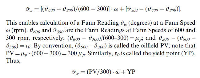
Shear rates in a drill pipe generally encompass the range from 511 to 1022 sec^-1 (Fann Speeds of 300 to 600 rpm), whereas in the annulus, flows are usually one to two orders of magnitude lower, such as 5.1 to 170 sec^-1 (Fann Speeds of 3 to 100 rpm). To change the Fann Speed to units of sec^-1, ψ (rpm) is multiplied by 1.7; to change the Fann Reading to units of dyne/cm^2, υ (degrees) is multiplied by 5.11. YP is actually in units of degrees but is usually reported as lb/100 ft2, since the units are
nearly equivalent: 1 degree=1.067 lb/100 ft2. Not only is the Bingham Plastic model easy to apply, it is also quite useful for diagnosing drilling fluid problems. Because electrochemical effects manifest themselves at lower shear rates, YP is a good indicator of contamination by solutes that affect the electrochemical environment. By contrast, PV is a function of the base fluid viscosity and concentration of solids. Thus, PV is a good indicator of contamination by drilled solids.
Application of the Power Law and Herschel-Bulkley Models to Rotary Viscometer Data
The Power Law model may be applied to Fann Readings of viscosity using the expression
Fann Reading = K * [Fann Speed]^n:
To obtain representative values of K and n, it is best to fit all of the Fann Readings to the model. A simple statistical technique, such as least squares regression, is quite satisfactory. If a programmable computer is not available but the flow regimen of interest is clearly understood, two Fann Readings will usually suffice to estimate the values of K and n. Naturally, this will lead to weighting of K and n to the Fann Speed range covered by those two Fann Readings. To estimate K and n in the simple
Power Law model from two Fann Readings, take the logarithm of both sides and substitute the data for the respective Fann Readings and Speeds:
Log (Fann Reading) = LogK + n Log (Fann Speed):
For example, assume pipe flow and a shear rate of interest covered by the 300 and 600 rpm Fann Readings. If the Fann Readings are 50, 30, 20, and 8 at 600, 300, 100, and 6 rpm, respectively,
Log [50] = LogK + n Log [600]
and
Log[30] =LogK + n Log [300].
Subtracting the second equation from the first eliminates K and producesone equation for n:
n= {Log [50/30]}=Log [600/300]= 0:737.
The value of K may be determined by substituting 0.737 for n in one of the equations above:

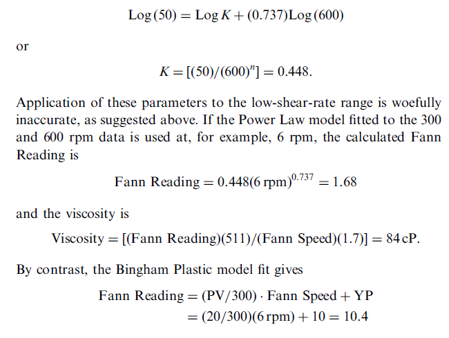
and the viscosity at 6 rpm is
Viscosity = {(Fann Reading)[511]=(Fann Speed)[1:7]} = 521 cP.
Thus, none of the rheology models should ever be used to extrapolate outside of the range used for the data fit.
The Herschel-Bulkley model is more difficult to apply, since the equation has three unknowns and there is no simple analog solution. Calculation of K, n, and ζ0 is generally carried out with an iterative procedure, which is difficult to do without a programmable computer. An alternative, which works fairly well, is to simply assign to ζ0 the 3-rpm Fann Reading, subtract that reading from all of the Fann Readings, and fit them to the Power Law model as described above.

CHARACTERIZATION OF SOLIDS IN DRILLING FLUIDS

Selecting, arranging, and operating solids-removal equipment to optimize the drilling-fluid cleaning process require accurate information about the intrinsic nature of the cuttings (drilled solids) and solid additives.
1. Nature of Drilled Solids and Solid Additives
Particle size, density, shape, and concentration affect virtually every piece of equipment used to separate drilled solids and/or weighting material from the drilling fluid. In the theoretically perfect well, drilled solids reach the surface with the same shape and size that they had when they were created at the drill bit. In reality, cuttings are degraded by physicochemical interaction with the fluid and mechanical interaction with other cuttings, the drill string, and the well bore.
Cuttings hydrate, become soft, and disperse in aqueous fluids and even in invert-emulsion NAFs with excessively low salinity. On the other hand, cuttings may become more brittle than the formation in highwater- phase-salinity NAFs and can be mechanically degraded by the action of the rotating drill string inside the well bore, particularly in deviated, slim-hole, and extended-reach wells. Cuttings are also degraded by mechanical action. Abrasion of the cuttings by other cuttings, by the steel tubulars, and by the walls of the well bore can lead to rapid comminution of the particles. In summary, cuttings recovered at the surface are generally smaller and frequently more rounded than at their moment of creation, depending on the nature of the cuttings themselves and the drilling fluid. Accordingly, the particle size distribution (PSD) seen at the flowline can range from near-original cutting size to submicron-sized particles.
The surface properties of the drilled solids and weighting material, such as stickiness and amount of adsorbed mud, also can play major roles in the efficiency of a rig solids-separation device. Large, dense particles are the easiest to separate using shale shakers, hydrocyclones, and centrifuges, and the differences in size and density among different types of particles must be well known to design the appropriate piece(s) of equipment for the separation process. Indeed, the optimum efficiency window for each device depends on all four of these parameters: concentration, size, shape, and density. Furthermore, since removal of some— but not all—particles is desirable, characterization of each and every type of particle with respect to those variables is critical. LCM serves as a good example of this. Usually economics dictates removal of large LCM along with cuttings using scalping shakers. Sometimes, however, large concentrations of LCM are required—as much as 50 to 100 ppb— in the circulating system. In such cases, a separate scalping shaker may be installed ahead of the regular battery of shakers to remove the LCM and recycle it back into the mud system [Ali et al ].
2 Physical Properties of Solids in Drilling Fluids
Particle sizes in drilling fluids are classified as shown in Table 2.2 [M-I llc]. PSD is measured using various techniques. For particles >45 mm diameter, wet sieve analysis is simple, accurate, and fast [API RP 13C]. Alternative methods include the American Petroleum Institute (API) sand test, which provides a measure of the total amount of particles >74 mm diameter [API RP 13B1]; microscopic image analysis, whose size limit at the low end depends on the type of microscope employed; sedimentation, for particles 0.5 to 44 mm diameter [Darley & Gray]; Coulter counter, for particles 0.4 to 1200 mm diameter [API RP 13C]; and laser granulometry (also called laser light scattering, diffraction analysis, and Fraunhoffer diffraction), for particles 1 to 700 mm diameter [API RP 13C].

With the Coulter counter, the solids are suspended in a weak electrolyte solution and drawn through a small aperture separating two electrodes, between which a voltage is applied and current flows. As each particle passes through the aperture, it displaces an equal volume of conducting fluid and the impedance between the electrodes increases in a manner that can be correlated with the particle size.
Laser granulometry is rapidly gaining popularity as the method of choice for PSD measurements. In laser granulometry, the solids are dispersed in a transparent liquid and suspended by circulation, if necessary, the slurry may be viscosified with a material like xanthan gum polymer. A beam of light is shone on a sample of the suspended solids, and the intensity versus the angle of the scattered light is analyzed to determine the PSD. Freshwater is used to disperse inert materials like barite. The drilling-fluid base fluid (saltwater, etc.) is used for all other solids (e.g., drilled solids). The sample is diluted to make it sufficiently transparent to obtain accurate readings. The instrument fits the particles to a spherical model to generate a histogram of number of particles versus particle size. For particles that do not fit a spherical model very
well, such as plates or rods, calibration with a known PSD of those particles is preferable. Laser granulometry results also depend on the step size chosen—for instance, for step sizes of 5 mm versus 10 mm, using 5 mm will generate two peaks that are each about half the size of a peak generated using 10 mm. If the step size chosen is too large, the reported PSD may miss some of the fine structure of the spectrum; on the other hand, a step size that is too small will generate excessive oscillations and the spectrum will appear to be very ‘‘noisy.’’


Figure 2.6 shows typical laser granulometry PSD curves for feed, liquid effluent (overflow), and solids discharge (underflow) for a field mud processed by a centrifuge. The efficiency of the device may be calculated from these data. PSD curves for each piece of equipment allow a more detailed understanding of what the device is doing and whether the equipment is optimally configured for the fluid being processed. There are calls within the drilling industry now to make laser granulometers standard equipment on critical wells, particularly high temperature/ high pressure and extended-reach wells, where the equivalent circulating density (ECD) is likely to exceed the fracture gradient.
Adsorbed mud, as well as swelling and/or dispersion of the cuttings resulting from interaction with the mud, can affect the PSD of cuttings. Comminution (degradation) of drilled solids has a strong impact on rheology and the total amount of mud adsorbed on the solids, inasmuch as the forces between the particles and the amount of mud adsorbed on them is proportional to their surface area. Drilled solids generally become comminuted while in the well bore and mud pits, as well as during passage through solids-control devices, through abrasion and chemical interaction with the base fluid. Surface-area increase due to comminution is proportional to the decrease in particle diameter. For example, breaking up a 100-mm-diameter particle into 5-mm particles will increase the total surface area by a factor of 20. Consequently, the
amount of mud adsorbed on the solids in this case will increase roughly by a factor of 20 as a direct result of comminution. Low-shear-rate viscosity will also increase significantly with this increase in total surface area, though the relationship is not strictly linear.
Average particle density, also termed ‘‘true’’ or ‘‘intrinsic’’ density, has units of weight/volume. Specific gravity (SG) is the ratio of the density of the material in question to the density of water and is, of course, unitless. Since the density of water is close to 1 g/cm3 over a wide range of temperature and pressure, the values reported for average particle density and SG are essentially the same. Average particle density should not be confused with bulk density (as often given in the Material Safety Data Sheet), which is a measure of the density of the packaged material. The LeChatelier flask method is the standard for determination of the average particle density of barite and hematite [API 13A]. In this method, one measures the incremental change in volume accompanying the addition of 100 g of the weighting material to a precisely measured volume of kerosene. A more convenient, but less accurate, method for determining density of weighting materials is the air pycnometer
[API RP 13I]. Another convenient method, which is rapidly gaining in popularity, is the stereopycnometer [API RP 13I]. In contrast to the air pycnometer, the stereopycnometer is as accurate as the LeChatelier flask method, and it can be used to measure density of any kind of particulate, including drilled cuttings. The stereopycnometer employs Archimedes’ principle of fluid displacement (helium, in this case) and the technique of gas expansion [API RP 13I].
Particle shape, partly described by the so-called aspect ratio, is not fully quantifiable. Neither is it possible to incorporate the broad spectrum of particle shapes in drilling fluids into particle-separation mathematical models. At this time, an old simple classification scheme is still used: granule, flake, fiber [Wright].
Concentration of particles in a mud is generally measured using aretort (an automatic portable still). The volume percentage of lowgravity solids (% LGS)—clays, sand, and salt—and the volume percentage of high-gravity solids (% HGS)—weighting material—are calculated from the measured volumes of the distilled fluids and the density of the mud. The calculated % LGS serves as an indicator of the effectiveness of the solids-control equipment on the rig. Occasionally both the overflow
and underflow solids from each piece of equipment are reported. Unfortunately, inaccuracies inherent in the retort, combined with the common practice of using an average density for the LGS and an average density for the HGS, can generate considerable uncertainties in % LGS. This is particularly true for low-density fluids, where a slight error in reading the retort will generate misleading—usually high— values of % LGS. However, if the calculated % LGS is below the target
limit (typically 5%), and dilution is not considered excessive, the solidscontrol equipment is considered to be efficient. (Calculation of solidsremoval
efficiency is presented in Chapter 15 on Dilution.) It should be noted that % LGS includes any clays that are purposefully added to the drilling fluid (for viscosity and filtration control). If a fluid contains 20 lb/bbl bentonite, it already contains 2.2% LGS before it acquires any drilled cuttings; in such fluids, the target limit of % LGS may be somewhat higher than 5%.
Concentration of particles affects mud properties, particularly rheology, which in turn affect the amount of residual mud on drilled solids. For noninteracting particles, the Einstein equation describes the effect of particles on the effective viscosity, μe, fairly well:

where μ is the viscosity of the liquid medium and μ is the volume fraction of the inert solids. This effect is independent of particle size, as long as the particles are suspended in the medium. The Einstein equation represents the effect of ‘‘inert’’ particles like barite fairly well, at least until their concentration becomes so great that the particles begin interacting with each other. Most particles in drilling fluids, however, have strong surface charges and interact strongly with each other at any concentration. Since all particles are enveloped by drilling fluid, attractive forces among strongly interacting particles (e.g., clays, drilled solids) generally lead to higher internal friction, hence a higher viscosity. Repulsive forces, such as are generated in muds containing high levels of lignosulfonate or other anionic polymers, will tend to exhibit lower viscosity. Because of these attractive/repulsive forces, strongly interacting particles generate an internal ‘‘structure’’ in a fluid, which manifests
itself most clearly at low fluid velocities. Thus, in most drilling fluids, significant deviations from the Einstein equation are the norm, as is discussed in more detail in the next section.
The viscosity of a drilling fluid must be maintained within certain limits to optimize the efficiency of a drilling operation: low-shear-rate viscosity needs to be high enough to transport cuttings out of the hole efficiently and minimize barite sag, while high-shear-rate viscosity needs to be as low as possible to maintain pumpability, remove cuttings from beneath the bit, and minimize ECD of the mud. In an analogous manner, for efficient operation of solids-control devices, the concentration
of drilled solids needs to be maintained within a specified range [Amoco]. The upper end (e.g., 5%) is particularly important, but the lower end (typically higher than 0%) is also important for most devices.
Stickiness of cuttings and its effect on the performance of solidscontrol devices are only beginning to be investigated. Various properties of the mud, along with lithology of the formation being drilled, are known to affect stickiness of particles, especially cuttings [Bradford et al.]. Generally, separation efficiency of any solids-control device decreases with increasing stickiness of the cuttings. Rheology, shale inhibition potential, and lubricity of the mud all can affect the stickiness of particles, which in turn affects performance of solids-control equipment, especially shale shakers. To handle gumbo (very sticky cuttings consisting primarily of young water-sensitive shale), operators will install special gumbo removal devices ahead of the shakers. To aid in conveyance of gumbo, the shaker screens are kept wet with a fine mist and
angled horizontally or downward toward the discharge end. Gumbo cannot be transported effectively on a linear motion or balanced elliptical
motion screen that is sloped upward.