Design of Hydrocyclone for Drilling Solid Separation

Hydrocyclone, as in Fig. 1, is the device that is widely used for the separation of materials normally in the form of solid particles. In drilling rig business, it’s mainly used in solids control field. it’s main part of desander and desilter. The device can offers effective solid removal in a compact package comparing with other methods. The suspended solids are separated from the liquid due to the centrifugal force induced inside the hydrocyclone (Fig. 2). The bigger and heavier particles flows out along with the hydrocyclone wall towards the underflow pipe, while the smaller and lighter ones change their directions upwards when they approach the cone apex and flow out through the vortex finder. It has been used in many fields like dewatering of oil or gas and medicine liquid extraction from organic materials as well as liquid separation from solid materials.

There are two types of method to design an optimum hydrocylone. The first type is based on established empirical rules for specific materials handling. Although this may be adequate for conventional cyclone applications, it does not cater for unusual cyclone geometries or processes. The alternative is to use a CFD (computational fluid dynamics) model. This is a numerical solver for non-linear fluid flow equations and the hydrocyclone is actually a challenging flow problem although the structure is simple. CFD has been used effectively in many areas, but computational fluid modeling of the complex multi-phase flow in a hydrocyclone is not a trivial task. Most practical CFD modeling of cyclones has been limited to single phase flow calculations, so the separation efficiency is normally predicted using a Lagrangian particle tracking approach. However, hydrocyclone operates with solid volume fractions in excess of 10%. When high solid volume fractions occur, the Lagrangian approach is not suitable. Therefore, for the modeling of the multi-phase flow, Eulerian approach was chosen in this study. The approach of explicit
droplet integration of Lagrangian suffers when scaling to large three-dimensional flow situations. For this reason development in the past years has begun to focus on Eulerian schemes for simulating solidliquid two-phase flow.

NUMERICAL MODEL

The simulation analyses on the solid-liquid two phase flow have various analysis methods and differences of difficulty degrees according to solid distribution, and exchange degrees of mass, momentum and energy between solid and liquid, in which Euler and Lagrange methods are mixed and applied appropriately. Comparing the Eulerian multi-phase with the Lagrangian two-phase method, the former has the advantages if being computationally more efficient in situations where the phases are widely dispersed and/or when the dispersed phase volume fraction is high.

Recently, CD-adapco group released a new version of Star-CD capable of Eulerian multiphase flow modeling. In this study a set of distinct mass and momentum conservation equations is solved for each phase, and the phases are coupled via momentum transfer term. The pressure is assumed to be the same for all phases. In the following, we first present the fundamental equations for phase k (where k could be either the solid or liquid phase). The equations for the Eulerian twophase model are:

Continuity equation:

Formula (1)

where α^k is the volume fraction, ρ^k and v^k are the density and the phase velocity calculated by volumetric mean, respectively.

Momentum

Formula (2)

where τ^k and τ^tk are the laminar and turbulent stresses, respectively, p
pressure, M^k inter-phase momentum transfer per unit volume, int F^int is the internal force.

Turbulence

For a dilute fluid suspension, the incompressible Navier-Stokes equations by a suitable turbulence model are appropriate for modeling the flow in a hydrocyclone. Flow turbulence is modeled based on the k-ε model. The model consists of the turbulent momentum energy term(k) derived from rigid solutions and turbulent energy dissipation ratio(ε) calculated from physical inferences. Modified equations are solved for the first phase and the turbulence of the second phase is correlated using semi-empirical models. The additional terms account for the effect of particles on the turbulence field. Eq. (3) and (4) are the equations for continuous phase:

Formula (3) and (4)

where k^c and μ^c are the continuous phase turbulent kinetic energy and molecular viscosity, respectively. σk and σε are the turbulent Prandt number for k and ε equations. And the term S^k2 and S^ε2 represent two phase interactions.

Inter-phase Momentum Transfer

The momentum transfer term includes the drag, virtual mass and lift forces:

Formula (5)

For the drag force term, the most widely used formulae are the Ergrun equation for regions of high solid particle fraction and a modified Stokes’ law for regions of lower fractions.

Formula (6)

where α^tr is the transition volume fraction and usually 0.2. C^D is a drag force coefficient. A reasonably good approximation for the drag coefficient of spherical particles in the transitional region between the Stokes and inertial regime, 0.2< Re^d <1000, is the correlation of Schiller and Naumann(1993). Also, the results at low Reynolds number of Re^d ≤ 0.2 show a slight difference less than 5% with the correlation. So, in this study the drag coefficient for a spherical particle was obtained as below.

Formula (7)

The particle Reynolds number, Re^d is defined as

Formula (8)

The virtual mass force in Eq. (5) accounts for the additional resistance experienced by a solid acceleration. The lift force means the one that lifts up the solids when the continuous liquid flow field is non-uniform or rotational.

In general, the hydrocyclone consists of an overflow pipe, an underflow pipe, a vortex finder and a slurry feeding entrance, the sizes of which were determined by the previous design in order to apply to a sea test (Fig. 3). The solid concentration of feed was 10% by volume. The flow rates of inlet were 3 m/s and 5 m/s. The boundary conditions of overflow and under flow were set to atmospheric pressures. Turbulence kinetic energy and its dissipation rate are fixed by assuming a turbulence intensity of 5% and mixing length of 10%. Also, wall function was used to treat the turbulence of the wall area.

The finite volume mesh used for the calculation is shown in Fig. 3. A total 201,331 cells were generated for the simulation by applying extrusion and hybrid cell methods. The density of solid particles was set to 2,150 kg/m3 and the diameter was under 1 mm. The unsteadystate simulation was performed for 25 sec from the injection of solid particles with volume fraction of 10%.

RESULTS AND DISCUSSIONS

The calculated vector plot of the vertical and horizontal sections of the velocity is shown in Fig. 4 at the time of 20 s. The vertical section shows that flows along with the wall move downwards in the hydrocyclone. It is because heavier manganese particles approach the wall easily than water by the centrifugal force, which can be confirmed in the horizontal section. The predicted helical vortex field will clearly have an impact upon the particle separation performance and solids distribution within the hydrocyclone. After the manganese particles move toward the wall, they go down by gravitational force. On the contrary, an upward flow happens around the vortex finder, which is because all the injected slurry can not flow out of the underflow pipe and relatively lighter water flows upward due to the space decrease as the slurry moves towards the underflow pipe. As shown in Fig. 2, the envelop of zero vertical velocity can be observed in the vertical section in Fig. 4. For a long time, symmetry has often been assumed for the purpose of modelling and that is different from actual tests. As many researchers indicated, the velocity vector shows asymmetry from the axis of the hydrocyclone. From Fig. 4 and Fig. 5, it was shown that the presented hydrocyclone CFD predictions have provided a novel understanding of the development of the initial flow field.

Solid-liquid separation efficiency was analyzed for the feed velocity of 3 m/s as a reference case. Fig. 6 illustrates the solid volume fraction at the overflow and the underflow. At both outlets, the solid volume fraction increases rapidly from 2 second point after the hydrocyclone begins to operate. At the time it maintains less than 2% at the overflow pipe, while it is stabilized after about 15 sec, and maintains more than 58% of solid volume fraction at the underflow pipe, which shows that the manganese particle separation proceeds efficiently.

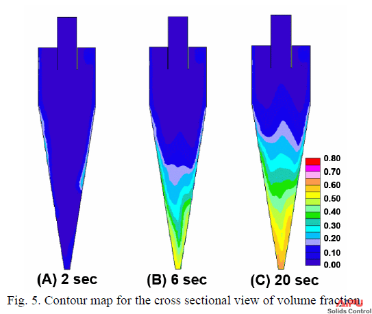
In Fig. 8, the solid volume fraction is illustrated according to time in the vertical section. At 2 second point, it is shown that the injected solid particles at the entrance flow along with the wall toward the underflow pipe. The particles show different distribution at both wall sides. It is because the inlet of the solids is positioned on the edge. The asymmetrical flow phenomena also occur at 6 and 20 sec. At 20 sec after the hydrocyclone operation, manganese particles accumulate up to the middle of the hydrocyclone. In Fig. 9, solid efflux at the overflow was represented to compare the case of feed velocity of 5 m/s with 3 m/s. From this, we can understand the effect of feed flowrate on the effluence of particles. At the time of 10 sec, the efflux values of solids were 0.45 kg/s and 1.71 kg/s. However, they were 2.74 kg/s and 3.74 kg/s at the underflow, which shows that the increase of flowrate can often cause bad recovery ratio from 79% to 68%. Also, the solid particles can not be discharged quickly through the underflow so it was shown that high flowrate can cause the blockade near the underflow. It was confirmed from the result that the appropriate feeding velocity should be investigated for a certain size of a hydrocyclone.

 

In addition to the numerical study, the test experiment was conducted so as to compare the results. The manufactured hydrocyclone was the same size with the CFD model of Fig. 3. Solid particles used were sands of 2,600 kg/m3 in density. The recovery was calculated by comparing the feed with the discharge at the underflow. That was over 90% much higher than the predicted recovery ration from the CFD model. It is speculated that the large difference between numerical and experimental results is caused by the heavier density and the bigger diameter of sands. So we need additional numerical and experimental studies.

CONCLUSIONS

In the study, we have tried to calculate the solid-separation efficiency by the commercial CFD model for the design and manufacture of a hydrocyclone. From the results, the following conclusions have been drawn:

1. A helical vortex is the most important factor to describe because it helps to separate solid and liquid from the slurry. In the study, a high Reynolds k-ε turbulent flow model was used to analyze the momentum between solid and liquid. Besides, Eulerian method was applied to describe solid-liquid two phase flow.
2. The flow phenomena analysis in the hydrocyclone shows that manganese particles moves along with the wall by centrifugal force toward the underflow pipe, and the relatively less dense water and fine particles flow adversely in the vortex finder and flow out toward the overflow pipe. The envelope of zero vertical velocity and the asymmetrical flow around the axis of the hydrocyclone were observed, as known in other previous experiments.
3. From the CFD results, it was shown that the solid particles were efficiently recovered, in which the solid volume fractions at the underflow and the overflow were maintained more than 58% and less than 2% respectively. At the time of 25 sec, solid recovery ratio at the underflow shows more than 75%, which is less than the result of a test experiment with sand particles of 2,600 kg/m3 in density.
4. When the basic design and the increased injection velocity 5 m/sec were compared, it was confirmed that when the injection velocity is higher, the recovered amount increases but the recovered ratio decreases because of the continuous accumulation of the manganese particles in the hydrocyclone. Therefore it was confirmed that the efficient injection flow velocity exists according to the size of the hydrocyclone.